Charts & Indicators

Technical analysis studies past prices and volume to forecast future price behaviour. In its traditional form it relies on visual pattern-reading, which (as the Market Theory page shows) is easily fooled by randomness. A data-driven trader uses the same tools differently: each indicator is a precisely defined feature computed from data, and its usefulness is an empirical question to be answered by testing.

Candlestick charts

Candlestick charts are usually traced to 18th-century Japanese rice markets, often attributed to the trader Homma Munehisa, and were popularised in the West by Steve Nison in the early 1990s. Each candle summarises one period (here, one trading day) with four prices:

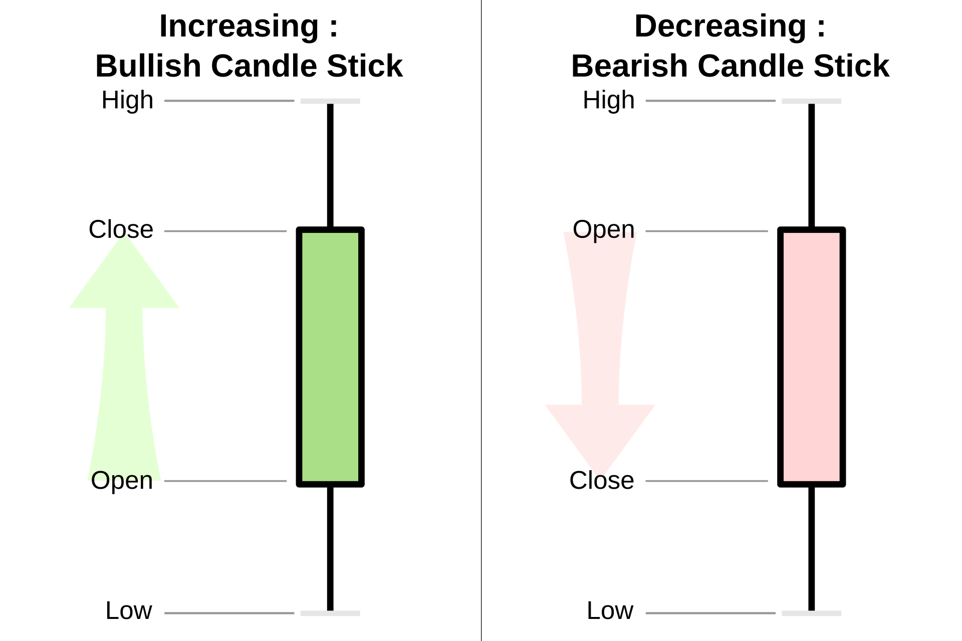
• Open and close form the body. On this site, a blue body means the close was above the open (an up day) and a red body means it closed lower.
• High and low form the thin wicks (or shadows) above and below the body.

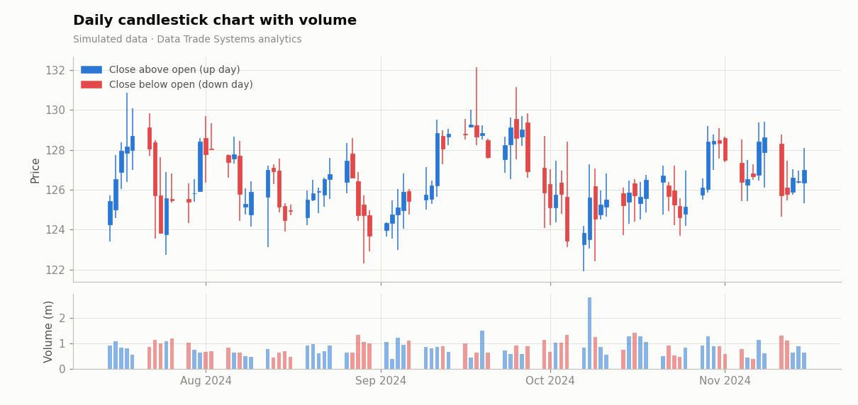
A candle compresses a day of trading into a shape that shows conviction (a long body), indecision (a small body with long wicks, called a doji) or rejection of a price level (a long wick). Volume, plotted beneath, shows how many shares changed hands, which indicates how much weight to give the move.

Moving averages

A moving average smooths noise to reveal the underlying direction. The two most common types are:

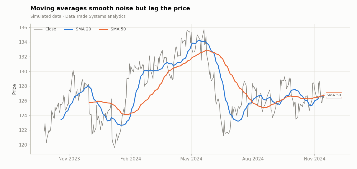
The simple moving average (SMA) weights the last n prices equally. The exponential moving average (EMA) weights recent prices more heavily, so it reacts faster. Every moving average involves the same trade-off: more smoothing means more lag. A 50-day average filters out more noise than a 20-day average, but it confirms a turn later.

import pandas as pd

def sma(close: pd.Series, n: int) -> pd.Series:
    return close.rolling(n).mean()

def ema(close: pd.Series, n: int) -> pd.Series:
    return close.ewm(span=n, adjust=False).mean()

Relative Strength Index (RSI)

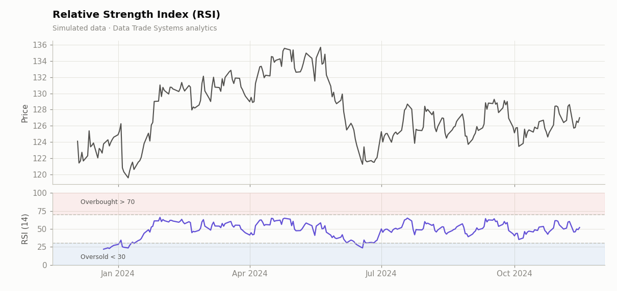
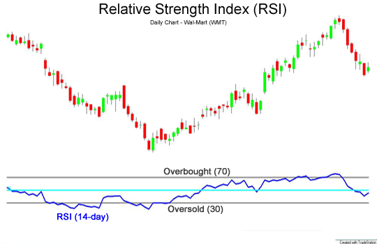
J. Welles Wilder introduced the RSI in his 1978 book New Concepts in Technical Trading Systems. It measures the speed of recent price changes on a 0–100 scale:

Wilder used n = 14 and smoothed gains and losses with his own exponential average (α = 1/n). Readings above 70 are conventionally called overbought and readings below 30 oversold. Despite the names, these levels are not reliable reversal signals on their own. In a strong trend the RSI can stay above 70 for weeks. Whether RSI extremes predict reversals is a testable, market-dependent question, which the Mean Reversion page examines.

MACD

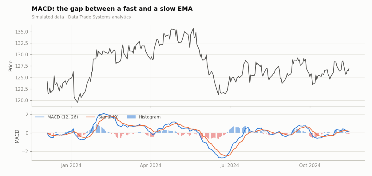
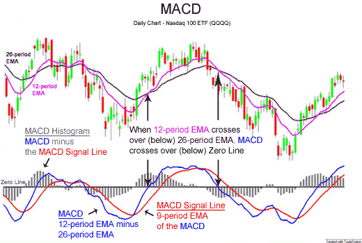
The Moving Average Convergence/Divergence indicator was developed by Gerald Appel in the late 1970s. It is the gap between a fast and a slow EMA, compared with its own moving average:

• MACD line = EMA₁₂ − EMA₂₆
• Signal line = EMA₉ of the MACD line
• Histogram = MACD − signal. Thomas Aspray added it in 1986 to show when the two lines are converging.

A positive MACD means short-term momentum is above long-term momentum. Crossings of the signal line are used as entry and exit triggers, and the histogram’s slope shows whether momentum is accelerating or fading.

Bollinger Bands

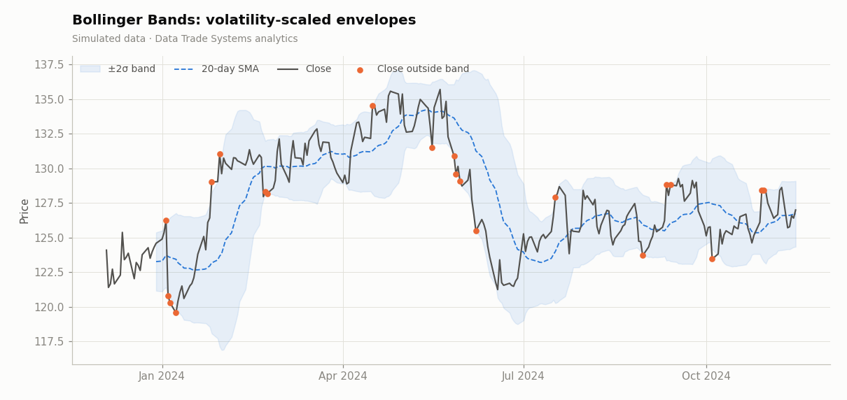
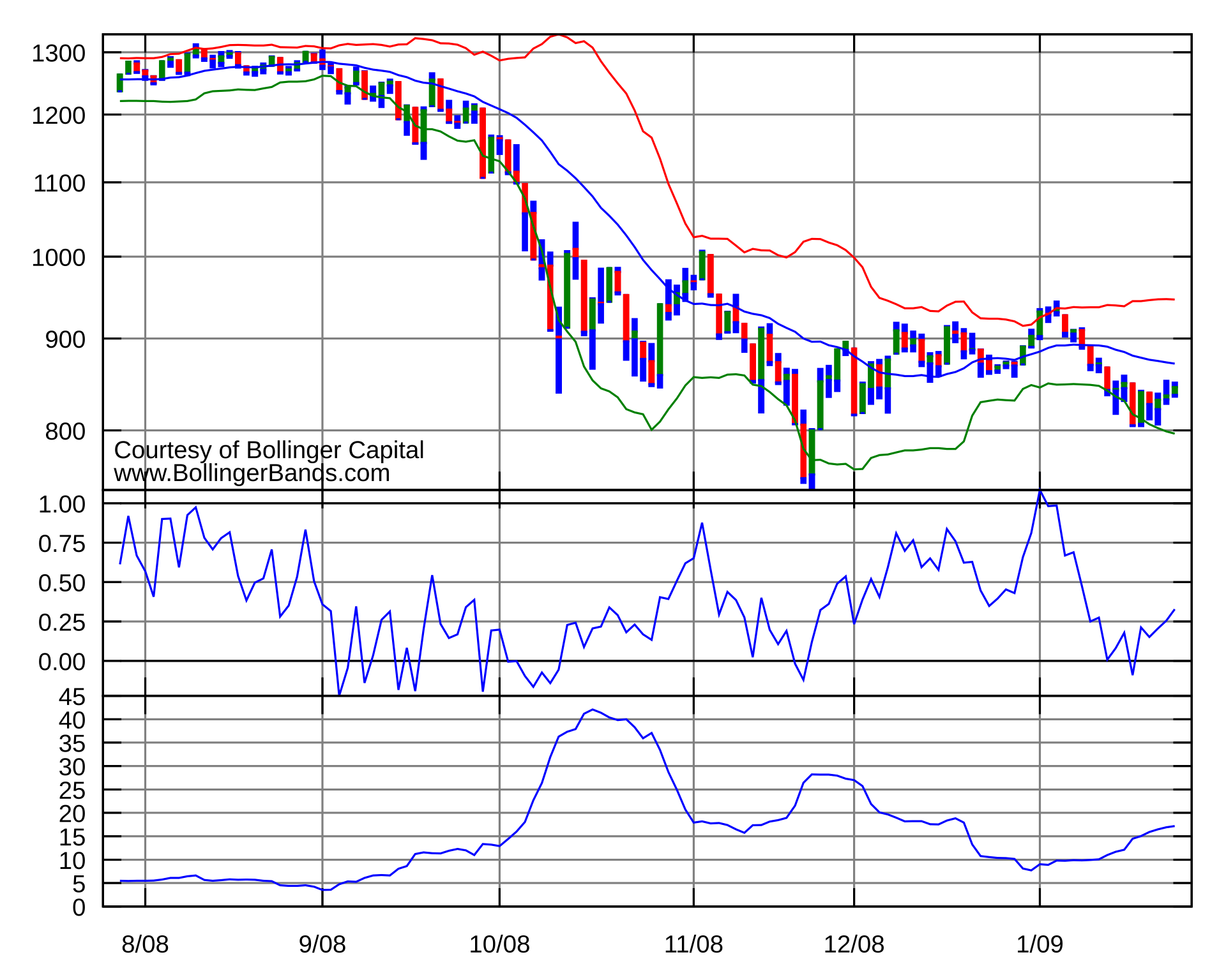
John Bollinger developed his bands in the 1980s to make trading envelopes adapt to volatility. They consist of a 20-day SMA with bands placed two standard deviations above and below it. When volatility rises the bands widen, and when markets are quiet they contract (a squeeze, often followed by a large move).

If returns were normally distributed, about 95% of closes would fall inside ±2σ bands. Because real returns have fat tails and trends, closes break outside more often than that, and how price behaves after a break is the basis of both breakout and mean-reversion strategies.

From indicators to features

Indicators become far more useful when you treat them as inputs to a model rather than as signals in themselves. A data-driven workflow looks like this:

1. Compute indicators using only past data at each point in time. A rolling window that includes today’s close cannot be used to trade at today’s open.
2. Normalise them so they are comparable across stocks and time, for example as distance from a moving average in units of volatility rather than in dollars.
3. Measure their relationship with future returns, using information coefficients, quantile sorts or simple regressions.
4. Combine the few that survive into a rule or model, and test it out of sample (see Backtesting).