Mean Reversion

Trend following bets that moves continue. Mean reversion bets on the opposite: that prices which stray too far from a “normal” level tend to come back. Both can be true of the same market at different horizons and in different regimes. Short-term reversals and medium-term momentum coexist in many equity markets, which is why a data-driven trader specifies the horizon before arguing about direction.

Why prices revert

• Liquidity provision: a large seller pushes the price below fair value temporarily. Whoever absorbs the order earns a premium when the price recovers.
• Over-reaction: investors extrapolate dramatic news, and prices overshoot before correcting. De Bondt and Thaler (1985) found that 3–5 year “loser” portfolios subsequently outperformed “winners”.
• Economic linkages: two companies exposed to the same drivers (two oil majors, or two share classes of one company) cannot drift apart indefinitely. Arbitrageurs pull them back together.
• Range-bound regimes: in the absence of news, prices oscillate within a range set by buyers and sellers who anchor on value.

The statistical counterpart is a stationary process, one with a stable mean and variance. A classic model is the Ornstein–Uhlenbeck process, in which the expected change is proportional to the distance from the mean. Its speed of reversion gives the half-life of a deviation, the most important number for deciding how long to hold a trade.

Strategy 1: Bollinger band reversion

Bollinger Bands (see Charts & Indicators) give a natural, volatility-adjusted definition of “too far”. The rule:

1. Buy when the close falls below the lower band (2σ under the 20-day average).
2. Short when the close rises above the upper band.
3. Exit when price returns to the middle band.

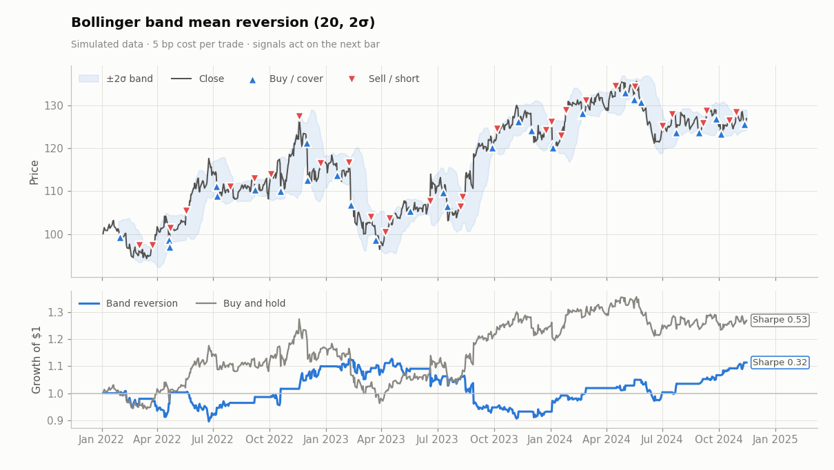
Compare this chart with the trend-following results on the same data. The reversion rule wins in ranging stretches and is badly hurt in strong trends, where “oversold” keeps getting more oversold. This is the core risk of mean reversion: a high win rate with occasional very large losses, the mirror image of trend following. Disciplined implementations add a time stop, a hard loss limit, or a regime filter that disables the strategy when a trend indicator is strong.

Strategy 2: RSI oversold / overbought

A popular short-horizon variant uses RSI extremes: buy when the RSI drops below 30, exit when it recovers to 50. Shorter RSI periods (2–5 days) produce more frequent, faster signals. Research by practitioners such as Larry Connors popularised two-period RSI rules on equity indices, an example of an edge that is plausible (short-term liquidity provision) yet must be re-validated because it is so widely known. You can test this rule with different thresholds in the Strategy Lab.

Strategy 3: Pairs trading and statistical arbitrage

Single-stock reversion is fragile because a stock’s “fair value” can genuinely change. Pairs trading sidesteps this by trading the relationship between two related stocks. The idea was developed in the mid-1980s by a quantitative group at Morgan Stanley led by Nunzio Tartaglia. Gatev, Goetzmann and Rouwenhorst (2006) later documented its historical profitability in US equities.

Cointegration

Two price series are cointegrated (Engle and Granger, 1987) if each wanders like a random walk but a linear combination of them is stationary:

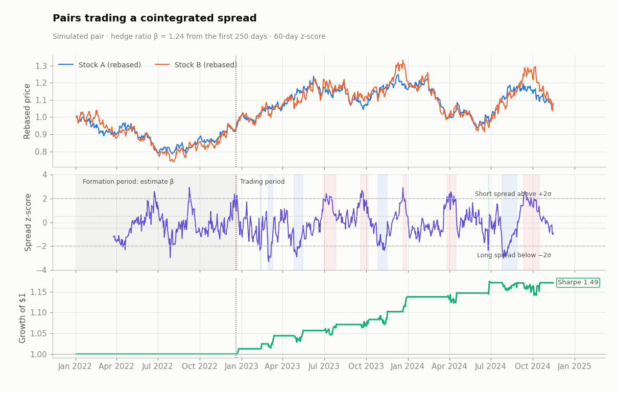
The hedge ratio β is estimated by regression on a formation period (here the first year) and then held fixed while trading. Re-estimating β every day is tempting, but because β multiplies the log-price level, small estimation errors can swamp the spread itself. The spread is standardised into a rolling z-score, and the trading rules are then simple:

• z > +2: the spread is rich, so short B, long β·A.
• z < −2: the spread is cheap, so long B, short β·A.
• |z| < 0.5: the spread has normalised, so close the trade.

import numpy as np

la, lb = np.log(pair["a"]), np.log(pair["b"])
form_a, form_b = la[:250], lb[:250]                    # formation period
beta = form_b.cov(form_a) / form_a.var()               # OLS hedge ratio, then fixed
spread = lb - beta * la
z = (spread - spread.rolling(60).mean()) / spread.rolling(60).std()

Because the position is long one stock and short the other, the market’s overall direction largely cancels out. The strategy is close to market-neutral: its returns come from the spread, not from the market.

Testing before trading

• Use a formal test (Engle–Granger two-step or Johansen) on a formation period, then trade on a separate trading period. Selecting pairs and measuring their profits on the same data is look-ahead bias.
• Screen many candidate pairs and you will find “cointegrated” ones by chance. Correct for multiple testing and require an economic link.
• Watch the half-life. Spreads that take months to revert tie up capital and are more likely to break.
• Relationships do break: a merger, a lawsuit or a change of business model can turn a stationary spread into a trend. Always cap the loss on a pair.