Before writing a single trading rule it helps to ask a harder question: why should prices be predictable at all? Financial economics has spent more than a century debating the answer. This page summarises the main ideas, because every strategy on this site is, implicitly, a bet about which of them is wrong, and when.
The efficient market hypothesis
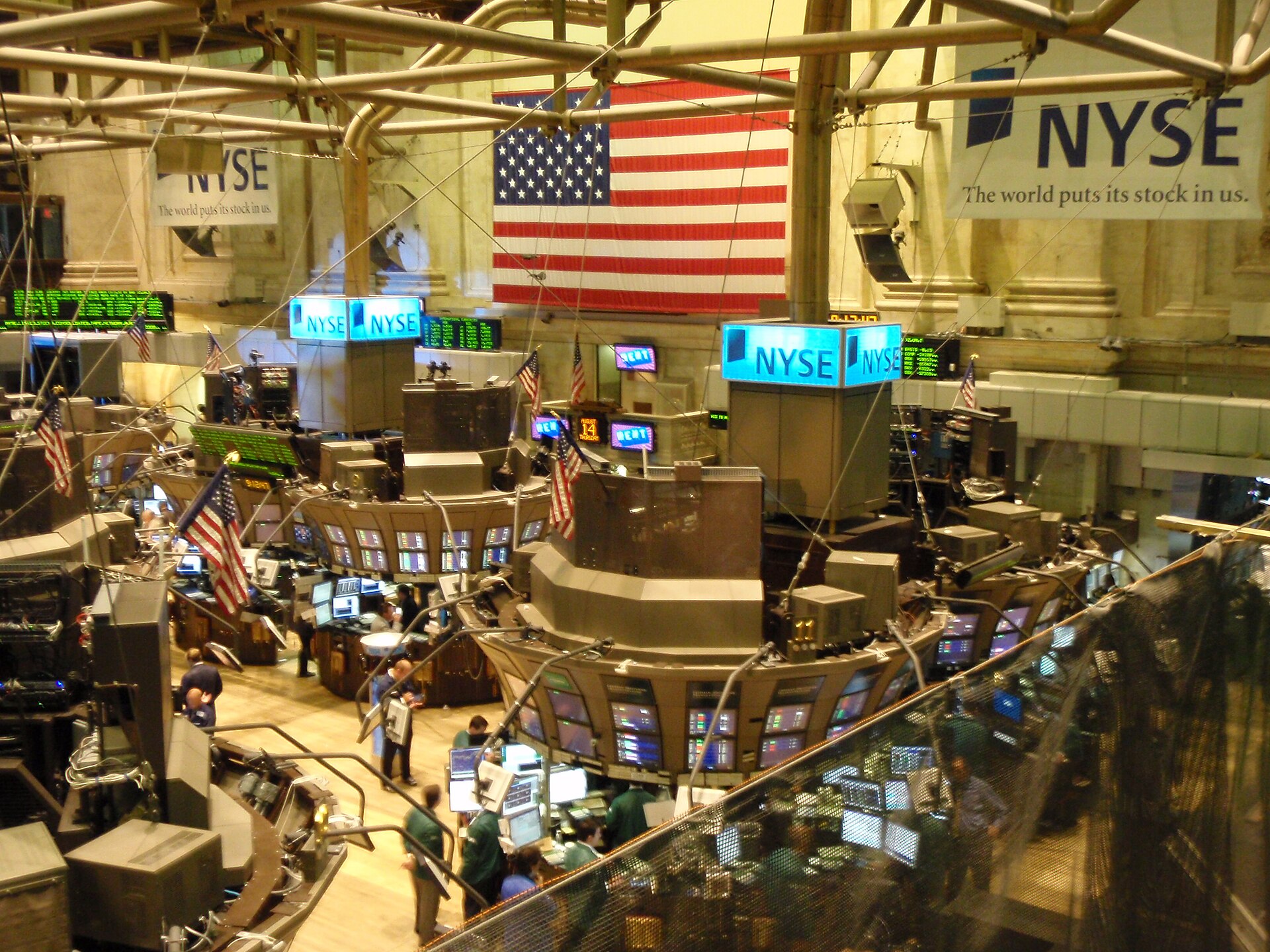
The efficient market hypothesis (EMH), formalised by Eugene Fama in his 1970 review of the evidence, states that asset prices fully reflect the information available to market participants. If that is true, no one can consistently earn returns above what is fair for the risk taken, because any exploitable information is already in the price. Fama distinguished three versions:
| Form | Information already priced in | Implication for traders |
|---|---|---|
| Weak | All past prices and trading volume | Technical analysis cannot earn excess returns |
| Semi-strong | All public information: prices, filings, news | Neither technical nor fundamental analysis can |
| Strong | All information, including private (insider) information | No one can, not even insiders |
The argument is economic, not mystical: if a simple pattern reliably made money, traders would exploit it until the pattern disappeared. Efficiency is therefore best understood as an equilibrium enforced by competition. That has an important corollary, first sharpened by Grossman and Stiglitz (1980): if markets were perfectly efficient, nobody would be paid to gather information, so nobody would gather it, and markets could not be efficient. Some inefficiency must survive to reward the people who keep prices honest.
Random walks
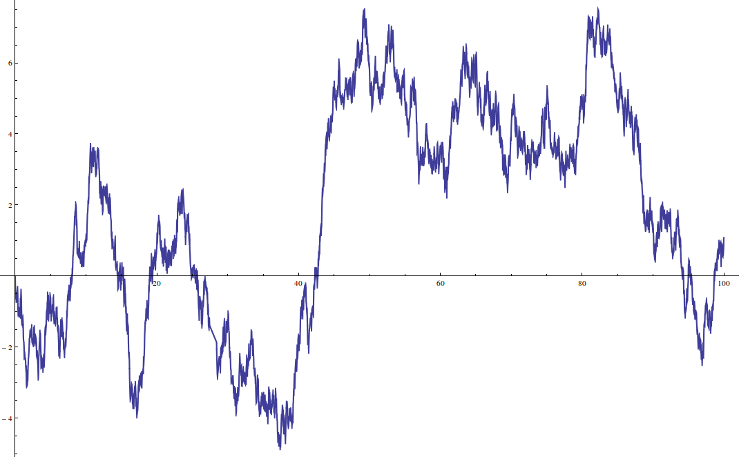
A closely related idea is the random walk hypothesis: successive price changes are independent, so the past path tells you nothing about the next step. Louis Bachelier modelled prices this way in his 1900 thesis Théorie de la spéculation, decades before the mathematics of Brownian motion became standard in physics. Burton Malkiel brought the idea to a general audience in A Random Walk Down Wall Street (1973).
The chart below makes the point visually. The grey lines are pure random walks, coin flips with a slight upward drift. The blue line is a simulated stock with genuine regimes (trending, ranging and volatile phases). By eye, the random walks show “trends”, “support levels” and “breakouts” just as convincingly as the series that actually has structure.
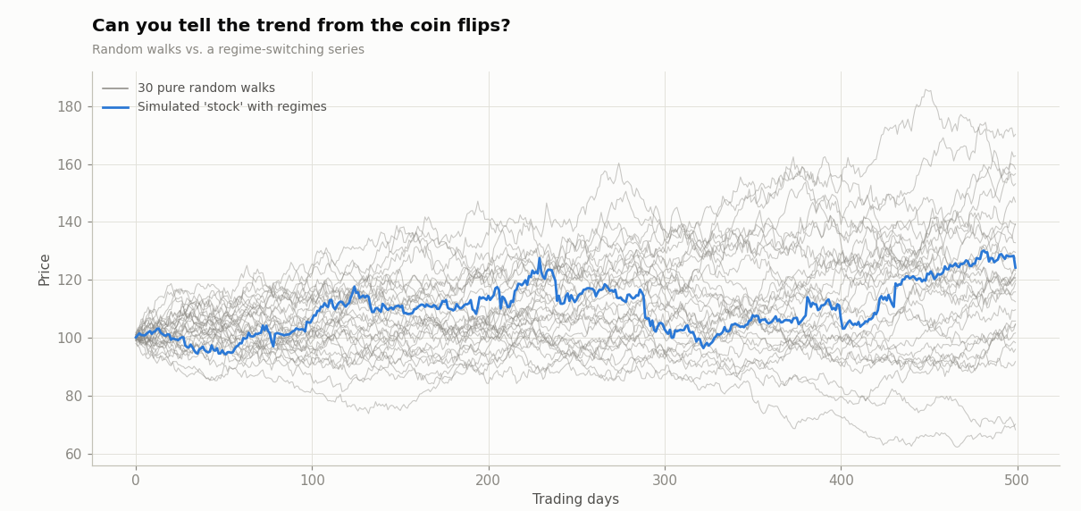
This is the first lesson of data-driven trading: human pattern recognition is not evidence. A pattern only counts if it survives a statistical test against the hypothesis that prices are random.
Testing for randomness
Researchers test the random walk hypothesis in several ways:
- Autocorrelation: are today’s returns correlated with yesterday’s? Under a random walk, autocorrelations at every lag should be indistinguishable from zero.
- Variance ratios: under a random walk, the variance of k-day returns is k times the variance of 1-day returns. Lo and MacKinlay (1988) rejected this for weekly US stock returns, finding positive autocorrelation, especially among small stocks.
- Trading-rule tests: does a mechanical rule beat buy-and-hold after costs and after adjusting for risk? This is the approach used throughout this site.
Returns are not normally distributed
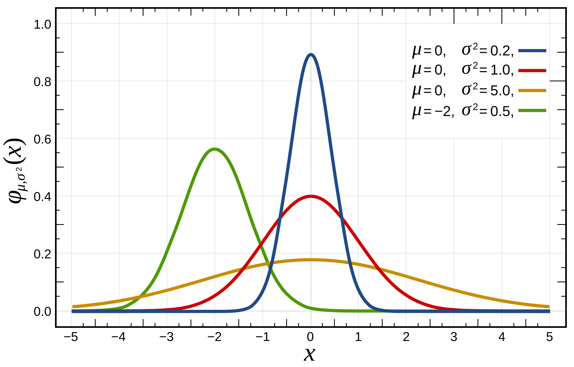
Many classical models assume that returns follow a normal (Gaussian) distribution. Real returns do not. In 1963 Benoit Mandelbrot showed that cotton price changes had far too many extreme moves for a bell curve, and the same is true of stocks: crashes such as October 1987, when US stocks fell more than 20% in a day, would be essentially impossible under normality.
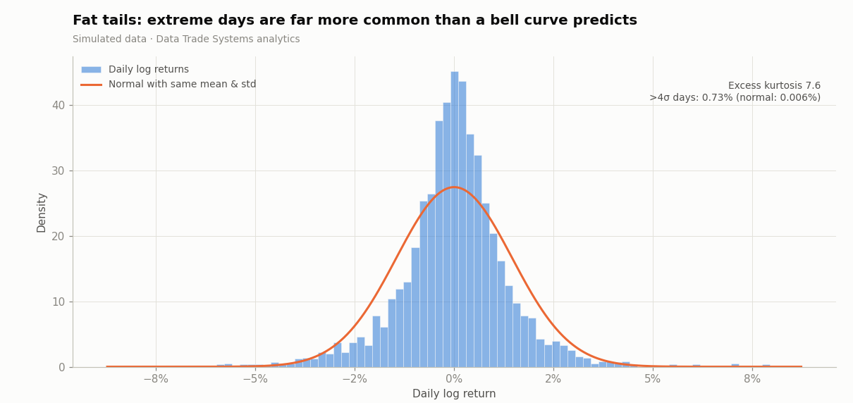
The histogram shows the typical shape: a taller, narrower peak and heavier tails than the normal curve. The statistic that measures this is excess kurtosis, which is zero for a normal distribution and clearly positive for equity returns. Two other stylised facts appear in almost every market:
- Volatility clustering: large moves tend to follow large moves, of either sign. Volatility is predictable even when direction is not, which is the foundation of the ARCH/GARCH models of Engle and Bollerslev and of the volatility-targeting techniques on the Risk Management page.
- Asymmetry: volatility tends to rise more after falls than after rises (the leverage effect), and crashes are sharper than rallies.
Practical consequence: any risk estimate built on a normal distribution (for example, a naive Value-at-Risk) will understate the probability of large losses. Data-driven traders use empirical distributions, stress tests and position limits, not just standard deviations.
Where do edges come from?
If markets are close to efficient, a strategy that earns persistent returns must be explained by one of three things. Knowing which one applies tells you how durable the edge is likely to be.
1. Risk premia
Some returns are compensation for bearing risk that other investors want to avoid. The equity risk premium itself is one example. Others include the value and size factors documented by Fama and French (1993), and the premium for providing liquidity during market stress. These returns can persist because they come with painful drawdowns at the worst possible times.
2. Behavioural biases
Behavioural finance, built on the prospect theory of Daniel Kahneman and Amos Tversky (1979), documents systematic departures from rational decision-making:
- Anchoring and under-reaction: investors update slowly to news, so prices drift in the direction of the surprise. This is one explanation for momentum and post-earnings drift.
- Herding and over-reaction: crowds extrapolate recent trends and then reverse, creating long-horizon mean reversion (De Bondt and Thaler, 1985).
- The disposition effect: investors sell winners too early and hold losers too long.
- Overconfidence: traders overestimate the precision of their information and trade too much.
3. Structural and institutional frictions
Index rebalancing, forced selling by leveraged funds, regulatory constraints, tax-driven trading and limits to arbitrage (Shleifer and Vishny, 1997) all create predictable flows. Such flows may be unprofitable for large institutions to exploit but available to smaller, more flexible traders.
The adaptive markets view
Andrew Lo’s adaptive markets hypothesis (2004) offers a synthesis. Markets are an ecosystem of competing strategies. Efficiency is not a fixed property but varies over time, rising as an edge is discovered and crowded out, and falling when conditions change or capital retreats. For a data-driven trader this has two practical consequences: edges decay, and a strategy’s performance depends on the regime it runs in. Both themes recur on the strategy pages that follow.
Next: the tools traders use to describe price behaviour, on the Charts & Indicators page.
Sources & further reading
- Wikipedia contributors, “Efficient-market hypothesis”, “Random walk hypothesis”, “Behavioral economics”, “Adaptive market hypothesis”, “Fat-tailed distribution”. Wikipedia, CC BY-SA 4.0.
- Fama, E. (1970). Efficient Capital Markets: A Review of Theory and Empirical Work. Journal of Finance 25(2).
- Grossman, S. & Stiglitz, J. (1980). On the Impossibility of Informationally Efficient Markets. American Economic Review 70(3).
- Lo, A. & MacKinlay, A. C. (1988). Stock Market Prices Do Not Follow Random Walks. Review of Financial Studies 1(1).
- Mandelbrot, B. (1963). The Variation of Certain Speculative Prices. Journal of Business 36(4).
- Lo, A. (2004). The Adaptive Markets Hypothesis. Journal of Portfolio Management 30(5).