Risk Management

A strategy’s signals decide what to trade. Risk management decides how much, and that is usually what determines whether a trader survives. Two people trading identical signals with different position sizes can end up with very different results: one compounding steadily, the other wiped out by a single bad month.

Measuring risk

Measure	Definition	What it misses
Volatility	Annualised standard deviation of returns: σdaily × √252	Treats gains and losses alike, and understates tail risk
Downside deviation	Standard deviation of negative returns only (used in the Sortino ratio)	Still a single number for a whole distribution
Value-at-Risk (VaR)	Loss not exceeded with, say, 99% confidence over a horizon	Says nothing about how bad the worst 1% is
Expected shortfall (CVaR)	Average loss in the worst x% of outcomes	Needs many observations of rare events
Maximum drawdown	Largest peak-to-trough fall in equity	Path-dependent, so one sample path is a noisy estimate

Drawdowns: the risk you actually feel

A drawdown is the percentage decline from the running peak of an equity curve. It is the number that ends careers and causes investors to abandon good strategies at the worst moment. The underwater chart below plots it over time:

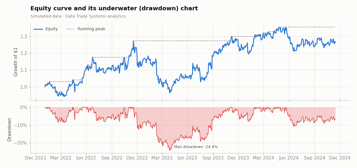
Drawdowns are asymmetric: losses need disproportionately large gains to recover.

Drawdown	−10%	−20%	−33%	−50%	−75%
Gain needed to recover	+11%	+25%	+50%	+100%	+300%

This is why professional risk managers set drawdown limits in advance, for example cutting position sizes by half after a 10% drawdown and stopping trading after 20%, and why they care about the length of drawdowns as well as their depth.

Position sizing

Fixed-fractional risk

The simplest professional rule: risk a fixed fraction of equity, often 0.5–2%, on each trade. If a stop-loss sits at distance d from the entry price, then

Position size then shrinks automatically after losses and grows after gains, and no single trade can do catastrophic damage. Using the Average True Range (ATR) to set d ties the stop to the market’s current noise level, which is how the Turtle Traders sized their positions.

Volatility targeting

Because volatility clusters (see Market Theory), recent volatility is a reasonable forecast of near-term volatility. Volatility targeting scales exposure inversely to it, so that the portfolio runs at a roughly constant level of risk:

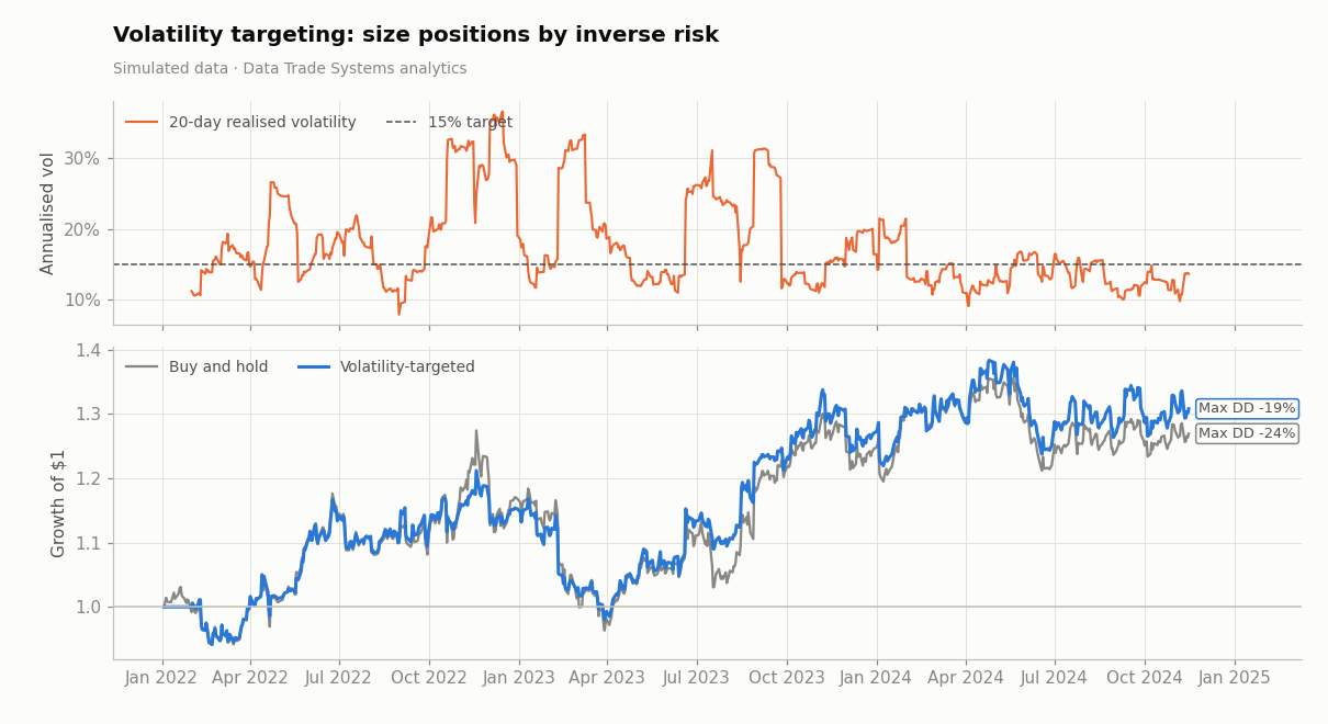
When markets become turbulent the strategy steps back, and when they are calm it steps up. Moreira and Muir (2017) found that volatility-managed versions of common factor portfolios improved risk-adjusted returns, because high volatility has not historically been matched by proportionally higher returns. The technique is widely used by trend-following and risk-parity funds.

vol = np.log(close).diff().rolling(20).std() * np.sqrt(252)
exposure = (0.15 / vol).clip(upper=2.0)        # 15% annual vol target, max 2x
# exposure is computed at today's close and applied from tomorrow

The Kelly criterion

In 1956 John L. Kelly Jr., a researcher at Bell Labs, derived the bet size that maximises the long-run growth rate of wealth. The mathematician Edward Thorp later applied it to blackjack and to markets. For a continuously traded asset with expected excess return μ and volatility σ, expected log growth at leverage f is

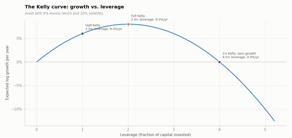
The curve shows three important facts:

• Growth peaks at full Kelly (here 2× leverage), but the peak is flat. Half Kelly earns three-quarters of the growth with half the volatility.
• At twice Kelly the expected growth rate falls to zero, despite a positive expected return on every bet. Beyond it, over-leverage guarantees long-run ruin.
• Kelly assumes that μ and σ are known exactly. In practice μ is estimated with huge error, so practitioners bet a fraction of Kelly. Over-estimating your edge pushes you to the right side of the curve, where risk rises and growth falls.

Diversification and portfolio construction

Harry Markowitz’s 1952 paper Portfolio Selection showed that what matters is the risk of the portfolio, not of each asset alone. Combining assets that are less than perfectly correlated lowers risk without lowering expected return in proportion. The set of best possible risk/return trade-offs forms the efficient frontier:

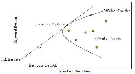
The same logic applies to strategies. Trend following and mean reversion tend to have low or negative correlation with each other. A portfolio of several modest, uncorrelated strategies usually beats a single “best” strategy on a risk-adjusted basis. The catch is that correlations are unstable and tend to rise towards 1 in a crisis, precisely when diversification is needed most.

A risk checklist

1. Define the maximum loss per trade and the maximum drawdown at which you stop, before you start.
2. Size positions by risk (volatility or stop distance), not by dollar amount.
3. Cap leverage well below full Kelly, and cap total gross exposure.
4. Limit concentration: per stock, per sector, and per strategy.
5. Stress-test with historical crises and with returns drawn from fat-tailed distributions.
6. Monitor live versus backtest performance and pre-commit to what divergence will make you stop.