Backtesting

A backtest simulates how a trading rule would have performed on historical data. It is the central tool of data-driven trading, and also the easiest one to misuse. A backtest is not a forecast. It is an experiment, and like any experiment it can be badly designed, run on biased data, or repeated until it produces the answer the experimenter wanted.

Anatomy of an honest backtest

1. Point-in-time data. At every simulated moment, use only data that was actually available then, including revised fundamentals, index membership and corporate actions.
2. Signal timing. A signal computed from today’s close can be traded at the earliest at today’s close (with slippage) or tomorrow’s open. The Data Trade Systems backtester applies every position from the next bar.
3. Realistic costs. Include commissions, the bid-ask spread, market impact, borrowing costs for shorts and financing for leverage.
4. A benchmark. Compare with a simple alternative, usually buy-and-hold, at equal risk.
5. Out-of-sample validation. Hold back data the strategy has never seen, and look at it once.

The classic biases

Bias	What goes wrong	Typical fix
Look-ahead bias	The rule uses information from the future, such as a centred moving average, the day’s close to trade at its open, or restated earnings.	Shift signals by one bar, and use point-in-time databases.
Survivorship bias	Testing only on stocks that exist today ignores those that went bankrupt or were delisted, which inflates returns.	Use a survivorship-free universe that includes dead stocks.
Data-snooping / overfitting	Trying many variants and reporting the best. The winner fits noise.	Hold-out data, walk-forward tests, multiple-testing corrections.
Cost underestimation	Zero or flat costs make high-turnover strategies look excellent.	Model spread and impact as a function of size and liquidity.
Regime bias	The test period happens to suit the strategy, for example a long bull market for a long-only rule.	Test across several market regimes and asset classes.

Here is how small the difference between a valid and an invalid rule can be in code:

# WRONG: today's signal earns today's return (look-ahead)
strategy_ret = signal * close.pct_change()

# RIGHT: yesterday's signal earns today's return
strategy_ret = signal.shift(1) * close.pct_change()

Overfitting: the central problem

Every parameter you tune and every rule you add or remove gives the backtest another chance to fit noise. With enough attempts, some variant will look excellent by pure chance. The chart below runs a grid search over dozens of moving-average crossover parameters. It measures each combination’s Sharpe ratio on the first 60% of the data (in-sample) and again on the remaining 40% (out-of-sample).

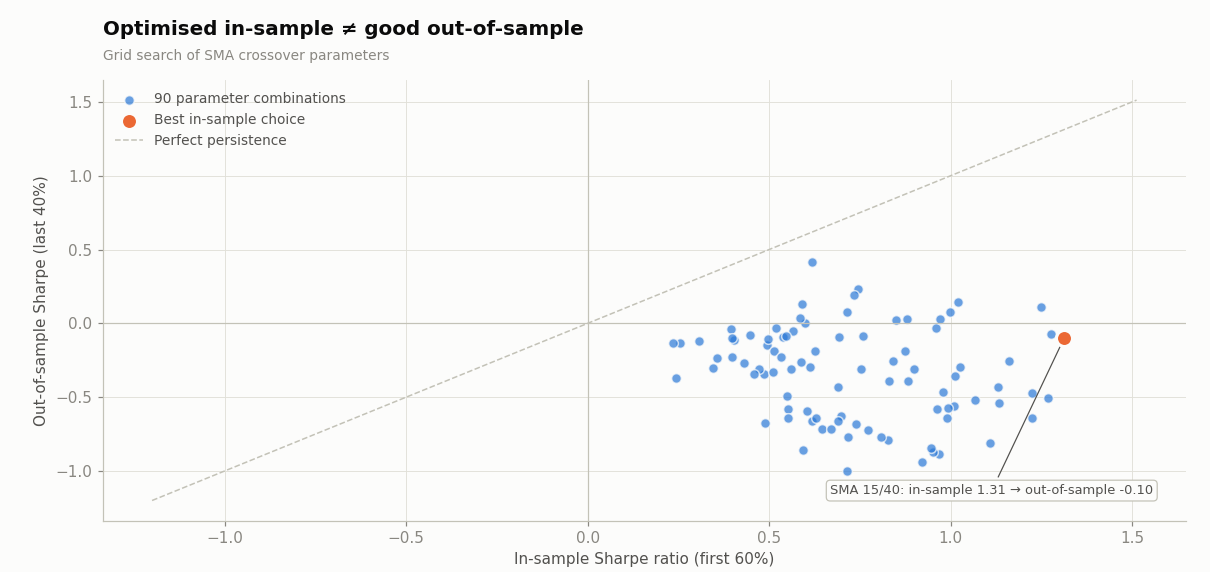
If in-sample performance carried over, the points would lie along the dashed diagonal. Instead they form a cloud, and the best in-sample combination (highlighted) has no special claim to the best out-of-sample result. Its in-sample performance was largely luck. This is selection bias under multiple testing, and it is the most common reason that strategies fail in live trading.

Walk-forward analysis

Walk-forward analysis turns a single train/test split into a rolling procedure that resembles how a strategy would actually be run: optimise on a window of past data, trade the next period with the chosen parameters, then roll forward and repeat.

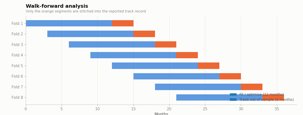
The stitched-together out-of-sample periods form a track record in which every trade used parameters chosen without knowledge of that trade’s outcome. If walk-forward performance is far worse than the full-sample optimum, the strategy’s apparent edge came from parameter fitting rather than from a real effect. Combinatorially purged cross-validation extends the idea by testing many train/test combinations while purging overlapping observations, which avoids leakage when labels span several days.

Reading the metrics

Metric	Formula	Rule of thumb
CAGR	(Final / Initial)1/years − 1	Meaningless without the risk taken to get it
Sharpe ratio	Annualised mean excess return / annualised volatility (Sharpe, 1966)	Above 1 after costs is good. Above 3 in a backtest usually means a bug or overfitting.
Sortino ratio	Mean return / downside deviation	Useful when returns are skewed
Max drawdown	Largest peak-to-trough decline	Expect live drawdowns to exceed the backtest’s
Calmar ratio	CAGR / |max drawdown|	Return per unit of pain
Exposure & turnover	Time in market, and trades per year	High turnover magnifies cost errors

A Sharpe ratio estimated from a few years of data is very uncertain. Its standard error is roughly √((1 + SR²/2) / years), so a Sharpe of 1.0 measured over 4 years carries a standard error of about 0.6. Short backtests can neither confirm nor rule out a modest edge.

From backtest to live trading

• Paper trade first to catch data, execution and timing problems.
• Scale in gradually and compare live fills with the backtest’s cost assumptions.
• Expect decay: published anomalies lose a significant part of their returns after publication (McLean and Pontiff, 2016).
• Keep a research log of every variant tried, so that you know your true number of trials.

Put these ideas into practice in the Strategy Lab. Change the market seed to see how much the same rule’s results vary across different simulated histories.